HIDE/UNHIDE ROW/COLUMNS IN EXCEL

Sometimes when you open an Excel file, you will notice that some columns are missing. This is one of the features to unhide and hide rows and columns in the worksheet without affecting calculations in any way.


Hiding rows and columns can be displayed in two ways:
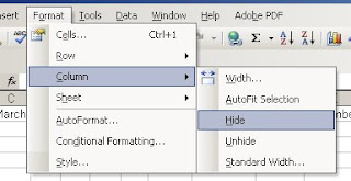
1. Select rows and columns that you wish to hide, and then go to Format -> Row or Column -> Hide.


2. Select rows and columns that you wish to hide, and then right click. Select Hide.


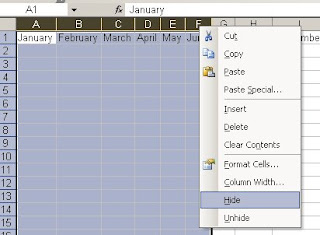
For displaying a hidden first column, it can be tricky if the hidden column is the left-most hidden column.
From the picture as below, notice that the month January to June is invisible.


To unhide the left-most hidden column(s), follow the steps below:
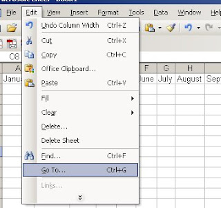
1. From the menu, click Edit -> Go To, or just press F5 will do.


2. A dialog box will be shown. In the Reference field, enter A1 (Column A Row 1).


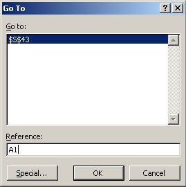
3. Click OK. Now cell A1 is selected (but because of column A is invisible, so you cannot see it on the screen).
4. From the menu, click Format -> Column -> Unhide.


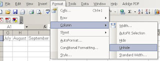
Notice that January now can be seen from the screen.


Another way to unhide the first column highlight the header of column B and drag to the very left of the spreadsheet until the gray block that marks the intersection of row and column headers, which mean column B and everything to its left (including the hidden column A) are selected.


Choose Unhide from the menu Format -> Column.